Saturday 23 September 2017

Parallel multivariate multiplication


Since my last blog on multivariate polynomial arithmetic, a lot has happened, so it's time to give an update, including our first parallel sparse multiplication benchmarks! In fact, there is so much to report that I'm restricting this blog to multiplication only!

The most exciting news since last time is that Daniel Schultz has gotten parallel sparse multiplication working. Daniel is the person we hired on the OpenDreamKit grant to work on parallel multivariate arithmetic. He's also implemented numerous improvements to the code, which I'll mention below.

After the last blog post, I discovered that a number of things affect the timings:

  • Polynomial ordering (lex, deglex, degrevlex)
  • Ordering of variables (x, y, z, t, u)
  • Whether one computes f*g or g*f, or in the case of division, p/f or p/g

Obviously in a perfect system, none of these would matter, but especially with our old code and with certain systems, they do. In particular, some of the division timings I gave previously for Flint, were invalid. I've now corrected them on the old blog.

In this blog, I will give new timings which always force lex ordering, for x > y > z > t > u, and will always take f*g.

Sdmp and Maple prefer deglex, so I will time these separately. We also don't have them available on our benchmark machine anyway.

Magma, Sage and Singular support a virtual panoply of orderings, whilst some systems are restricted just to lex or just to deglex. Flint supports lex, deglex and degrevlex. (Since there is no agreement on what revlex should be, we decided not to support it.)

We also discovered that we had implemented degrevlex incorrectly, and this has now been fixed. This didn't affect the timings in the last blog.

Sage division improvements


In the last blog we noted that Sage performed much worse than Singular for division over Z. The Sage developers immediately took note of this and set about fixing it. The latest release is 8.0 and it doesn't seem to have the fix, so we have to wait for the new version to give the new Sage division timings. It's great to see how quickly the community responded to this.

It was of course fixed by using Singular for that computation, rather than a very slow generic implementation of division.

Singular improvements


Hans Schoenemann has been working on improving the use of Factory from Singular. This means that Singular will call Factory for large arithmetic operations, since it is much faster. Singular itself is optimised for Groebner basis computations, not arithmetic.

The new improvements will currently take effect for computations with over 1000 terms or so, which is heuristically chosen to avoid overhead in converting to and from Factory's lex ordering and recursive polynomial format. Changing from an arbitrary ordering to a lex ordering and back can be extremely expensive, so this crossover is essential to avoid harming performance for smaller operations.

We've also decided that when we have a really solid, performant implementation of multivariate arithmetic, we are going to make use of it in Factory. The end result is that the code that we are writing now will be available to all Singular (and Factory) users.

The main operations that really benefit from such arithmetic are rational functions and multivariate factorisation. They aren't for speeding up Groebner Basis computations!

Flint improvements


Most of the actual work done on Flint since my last blog, has been done by Daniel Schultz. Here are some of the improvements:

Improved exponent packing


When using deglex or degrevlex, our monomial format packs the total degree field into the same words as all the other exponent fields. The trick of packing exponent vectors into bit fields goes way back to the early days of Singular. We get the idea from a paper of Hans Schoenemann.

Actually, Singular keeps the degree field separate from the rest of the vector (which in hindsight might have been a better thing for us to do as well), but we decided to try and pack it along with the other exponents.

The problem with our implementation of deglex and degrevlex is precisely this extra field that is required for the degree. If we don't want to overflow a word for each exponent vector, we have fewer bits per exponent when using degree orderings.

The maximum total degree is also often larger than the maximum of any individual degree, further exacerbating the problem. These issues mean that if we aren't careful, we can take more space for packed monomials using degree orderings than for lex orderings.

In practice, this meant that for our largest benchmarks, two 64 bit words were being used for exponent vectors, instead of one. This is because we were packing each exponent into a 16 bit field. Obviously six times 16 bits requires more than 64 bits.

We were using 16 bit fields, since we only supported fields of 8, 16, 32 or 64 bits (including an overflow bit), and 8 bit fields just weren't large enough; the maximum total degree in our largest benchmark is 160, (which requires 8 bits, plus an overflow bit).

We now pack into an arbitrary number of bits, and for 5 variables plus a degree field, it obviously makes sense to pack into 10 bit fields, since you get 6 of those in 64 bits. This is plenty big enough for all our benchmarks, in fact. The result is a 50% saving in time when using degree orderings.

Delayed heap insertion


Recently at ISSAC 2017 here in Kaiserslautern, Roman Pearce, one of the authors of the Sdmp library, told me about an improvement for multiplication that delays inserting nodes into the heap. In some cases, we know that they will be inserted at a later time anyway, so there is no hurry to put them in at the earliest possible opportunity, as this just increases the size of the heap.

Daniel implemented a version of this that he came up with, and it makes a big difference in timings, and shrinks the heap to a fraction of its original size.

Multi-core multiplication


Flint can now multiply sparse multivariate polynomials using threads. Daniel experimented with various strategies, including breaking one of the polynomials up. This strategy has the disadvantage of requiring a merge of polynomials from the various threads at the end, which is expensive.

The best strategy we found was to take "diagonals". That is, we divide the output polynomial up into chunks instead of dividing up the input polynomials. This has to be done heuristically, of course, since you don't have the output polynomial until it is computed.

This idea is contained in a paper of Jacques Laskar and Mickael Gastineau.

To ensure that all threads take about the same amount of time, we start with big blocks and take smaller and smaller blocks towards the end, so that no thread will be left running for a long time at the end while all the others are waiting. This gives fairly regular performance. The scheme we use is a variation on that found in the paper by Laskar and Gastineau.

The advantage of the diagonal splitting method is that no merge is required at the end of the computation. One simply needs to concatenate the various outputs from the threads, and this can be done relatively efficiently.

Improved memory allocation


At scale, everything breaks, and malloc and the Flint memory manager are no exception. I wrote a new memory manager for Flint which uses thread local storage to manage allocations in a way that tries to prevent different threads writing to adjacent memory locations (which would incur a performance penalty).

The design of this memory manager is beyond the scope of this blog, but it seems to work in practice. 

[A brief summary is that it allocates blocks of memory per thread, consisting of a few pages each. Each page has a header which points to the header of the first page in the block, where a count of the number of active allocations is stored. When this count reaches zero, the entire block is deleted. When threads terminate, blocks are marked as moribund so that further allocations are not made in them. The main thread can still clean thread allocated blocks up when their count reaches zero, but no further allocations are made in those blocks.]

The main advantage of this scheme, apart from keeping memory separated between threads is that we can block-allocate the mpz_t's that are used for the polynomial coefficients. This is critical, since in our largest benchmarks, almost a third of the time is spent allocating space for the output!

Unfortunately, each mpz_t allocates a small block of memory internally. That memory is handled by GMP/MPIR, not Flint, and so we still have 28 million small allocations for our largest benchmark!

I was able to make a small improvement here by changing the default allocation to two words, since we don't really use one word GMP integers in Flint anyway. But fundamentally, we are still making many small allocations at this point, which is very expensive.

This can be improved in a future version of Flint by setting a custom GMP memory allocator. But it will require implementation of a threaded, pooled, bump allocator. It can be done, but it will be a lot of work.

If we want to scale up to more than 4 cores (and we do!), we have no choice but to fix this!

Trip homogeneous format


Mickael Gastineau, one of the authors of Trip, was kind enough to send me a special version of Trip which allows access to their homogeneous polynomial format. It isn't optimised for integer arithmetic, but their papers show it is very fast for dense multivariate arithmetic, assuming you are happy to wait for a long precomputation.

The basic idea is to split polynomials into homogeneous components and precompute a very large table in memory for lookup. One only needs a table for the given degree bound, and Trip manages this automatically upon encountering this degree for the first time.

Before we get to the main timings below, we present Trip timings with this homogeneous format (excluding the precomputation).

We only time this for dense computations, since the precomputation is not practical for most of the sparse benchmarks. Moreover, since the code is not optimised for integer arithmetic, we use floating point to exactly represent integers, which means that the largest benchmarks can't be performed, since they would overflow the double precision floating point numbers.

Since Flint doesn't yet have parallel dense multiplication, these timings are restricted to a single core.


Dense Fateman (1 core)


New sparse multiplication benchmarks


In this section, we give timings for all systems (except Sdmp and Maple) on 1, 2 and 4 cores (where available). Most of the systems, including ours, perform badly on larger numbers of cores, unless the problems are really huge (> 30 minutes to run). When we have fixed our memory management issues, we'll do another blog post with timings on larger numbers of cores.

All the systems below were forced to use lexicographical ordering, with x > y > z > t > u, and we always take f*g (the polynomials f and g are the same length, so it's an arbitrary choice in reality).

The new delayed insertion technique Daniel implemented actually makes the timings for f*g and g*f the same for our new code. But other systems that support lex don't necessarily have this.

All of the timings in this section are done on the same machine, an old 2.2GHz Opteron server.

First, we give all the single core timings. We've added Piranha and Trip timings this time around. Incidentally, my understanding is that Piranha uses a hash table and therefore doesn't have a specific polynomial ordering. We include timings for Piranha to quench your burning curiosity.

Dense Fateman (1 core)


Sparse Pearce (1 core)


Of course, not all the systems can do parallel multiplication. So a smaller set of benchmarks for a smaller set of systems follows.

Sparse Pearce (2 core)

Sparse Pearce (4 core)

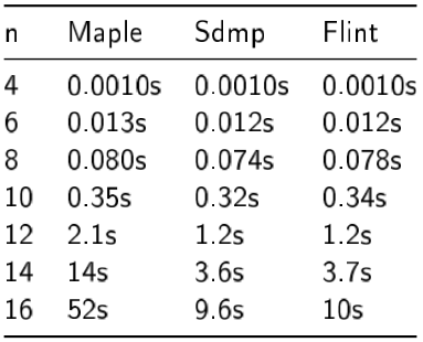
Sdmp and Maple 2017 timings


Michael Monagan very kindly granted me guest access to a machine that has Maple 2017 installed, which is currently also the only way to time Sdmp. Roman Pearce has also kindly given lots of information on how to use Maple and Sdmp, so that we can get fair timings.

The first thing to note is that the timings here are on a completely different machine to the above. So they are not in any way comparable.

I believe Sdmp internally only supports deglex. Therefore, we decided it best to use deglex for the Maple and Sdmp timings, otherwise we may be comparing apples and oranges. This is another reason one can't make a direct comparison with the timings for the other systems above. It also means there are no dense benchmarks, since our dense code doesn't support deglex efficiently yet.

It's also very important to point out that we have no way to run Sdmp except via Maple. We don't always get the timings for Sdmp below in practice, they are simply the self-reported times for Sdmp as a component of the full Maple run times.

It's not entirely clear why Maple is so slow on large inputs. Maple makes use of a DAG structure for its symbolic engine, rather than directly manipulating Sdmp polynomials. Something is apparently causing this to be incredibly slow when the polynomials are large. According to the Maple CodeTools it seems to be doing some long garbage collection runs after each multiplication. One wonders if there isn't something better that Maple can do so that their users can take practical advantage of the full performance of the Sdmp library in all cases!

An important benchmarking consideration is that for Maple, all Sdmp computations can be considered static. This means that Sdmp can block allocate their outputs, since the coefficients will never be mutated and therefore will never be reallocated. To simulate this, when comparing Sdmp and Flint, we write Flint polynomials into an already allocated polynomial. This probably slightly advantages Flint in some cases, but since we don't actually get the stated Sdmp timings in practice, this seems reasonable.

Of course, this isn't fair to Maple, but we are talking about a few percent, and the comparison with Sdmp was more interesting to us, since it is a library like Flint.

When comparing against Maple, we do the Flint timings using Nemo, which is a Julia package that wraps Flint. The code isn't on by default in Nemo, since we don't yet have GCD code, for example, but we switch the Flint code on in Nemo for the basic arithmetic timings in this blog. 

We take considerable care to ensure that both Maple and Sdmp use the same effective variable order that we do.

Sparse Pearce (1 core)


Sparse Pearce (2 core)


Sparse Pearce (4 core)

Conclusion


The project is coming along nicely. 

Daniel has started working on arithmetic over Q, and we'll update everyone when that is working. Hopefully we'll also find a good strategy for parallelisation of dense multiplication.

I should point out that the code described in this blog is very new, and after the last blog, we found many things that changed the results. We've taken much more care this time, but even an infinite amount of effort won't avoid all possible sources of error. The code itself is merged into trunk, since we mostly trust it, but it should still be considered experimental until it settles a bit.

I wish to thank Roman Pearce, Michael Monagan and Mickael Gastineau who have very generously provided details of how to use their systems, and gave us access so that we could do timings. There is an academic version of Trip available, which has everything but the homogeneous algorithm. For that, Mickael prepared a special version we could make use of.

We also want to thank the EU for their Horizon 2020 funding of the OpenDreamKit project.

Saturday 5 August 2017

Oscar:Antic Update


This week we had the first OSCAR:Antic workshop and coding sprint [1]. We had about 10 people turn up, though unfortunately we clashed with big meetings in Atlanta and Leiden. Still, we got a lot done, so we'll probably have another one of these soon!

For those who don't know, OSCAR is the computer algebra system being developed as part of a large DFG (German Research Council) transregional grant. The Antic subsystem of OSCAR is the Number Theory subsystem, consisting of Julia packages such as Hecke.jl, Nemo.jl and making use of Flint, Arb, the Antic C library, etc.

The workshop and expenses for invited speakers were funded by DFG TRR 195, but I should also note that a number of the participants are currently employed by OpenDreamKit, an EU Horizon 2020 grant.

Fp bar


The focus of the workshop more or less ended up being finite fields and their embeddings. Luca De Feo gave a really fantastic set of talks on algorithms for embedding finite fields with the aim of eventually reaching an implementation of Fp bar (the algebraic closure of the finite field of p elements).

We learned about all the recent breakthroughs in using elliptic curves over a finite field to efficiently do such constructions, including the papers of Luca and his coauthors [3].

Luca put all this work in the context of the older work of Bosma-Cannon-Steel and Lenstra-deSmit and the algorithms of Allombert and Plesken.

One of the main aims of the coding sprints was to implement a naive embedding method in Nemo, which just relies on finding roots of one finite field in another. This is still work in progress, but I think it is fair to say we made some good progress towards this.

The eventual aim is to have a modern sophisticated and highly performant implementation in Nemo, based on the code of Luca and his student Jean Kieffer. Some of the basic building blocks for this will be in Flint, of course.

The basic steps were:
  • Add some additional helper functions to Flint
  • Add root finding, based on equal degree factorisation, to Flint
  • Port the Hecke code for maps into Nemo
  • Add the code for handling embeddings, going up and down along embedding maps
  • Thinking about how to handle compatibility
  • Designing an interface for Nemo

Elliptic curve cryptography in Nemo


Luca and Jean presented a poster at ISSAC, which was held the previous week in Kaiserslautern. I think they even won an award for their poster.

Following on from this, Jean gave a talk at our Antic workshop on the work he and Luca have been doing on a Nemo module for elliptic curves over a finite field [4]. You can find the slides on the workshop homepage [1].

One remark that I found interesting was a note Jean made on performance. One of his graphs showed that Sage was beating Nemo for a generic implementation of Weierstrass elliptic curves over a finite field of cryptographic sized characteristic (e.g. p = 2^502 + 49), especially as the degree of the field grows.

We eventually traced this down to two specific things:

  • Sage was using one division instead of two in its implementation of the addition law on an elliptic curve (this was easily fixed in Jean's code)
  • Sage was using Pari for finite fields, and Pari is really fast at finite field arithmetic
My contribution was to speed up arithmetic for finite fields of smallish degree for large characteristic. Addition is still faster in Pari, due to their stack based memory management, but we now have multiplication that is faster than Pari, inversion about the same speed (sometimes faster, sometimes slower, to within about 1-2%), division and powering faster than Pari.

The tricks involved in speeding up inversion (and hence division) were as follows:

  • Improvements to the memory manager in Flint to block allocate mpz_structs
  • implement a gcdinv function for the Flint fmpz_mod_poly module (polynomials over Z/pZ for large p), instead of using the xgcd implementation, which does additional work
  • use temporary allocations (on the stack where possible) throughout the gcdinv and divrem code
  • delay reduction mod p in the divrem_basecase code in fmpz_mod_poly
  • inplace divrem_basecase
  • change crossover to divrem_divconquer to a higher value, in light of new basecase improvements
These improvements dropped the time for inversion in a finite field of degree 5 in large characteristic from about 12.7s for 100,000 inversions to about 8.7s.

There's still one potential improvement we could make, which would speed things up quite a bit:

  • implement a dedicated gcdinv function that doesn't call out to divrem, but does division itself, delaying reduction all the way through the entire Euclidean algorithm, except when actually needed
This would be quite a lot of work and so we didn't implement this yet. Contributions welcome.

An interesting observation


Initially we believed that Pari has special code for quadratic extensions of Fp. This is because we were constructing Fp^2 and then inverting f = x^1234 as a benchmark for inversion.

After investigating this, I realised that Pari was using cyclotomic polynomials for at least degree 2 and 4 extensions, where possible. This meant that in the degree 2 case, x^3 = 1 and in the degree 4 case x^5 = 1.

Of course x^1234 is not a really random looking element in such extensions, and it just so happens that the extended gcd computation that is necessary for inversion really goes fast for such computations.

I don't see how to make use of this in general, but it was interesting that it made such a huge difference (a factor of 10 or so in Pari).

Actually, we don't yet get such an improvement in Flint (it's more like 5x), so I will look into that today. It's almost certainly due to not terminating the xgcd early enough, or not handling a leading coefficient of 1 optimally, or something like that. It'll be something trivial, but worth optimising for, I think.

Update 06 Aug: this is now fixed in flint/trunk. It was indeed due to not dealing with length 1 remainders in a special case in the gcdinv code.

Other topics


Many other topics were covered at the workshop.

Ball arithmetic


Fredrik Johansson gave a very nice presentation on Arb for ball arithmetic over R and C. The slides are on the workshop website [1].

Generic polynomial testing


We decided to write test code for generic polynomials in Nemo. Three of us (me, Luca and Remi) wrote test functions, with particular emphasis on:

  • towers of univariate polynomial rings
  • generic polynomials where the base ring is built over a characteristic p field
  • randomised tests
As expected, this turned up numerous corner cases and failures, most of which are fixed (the rest will be fixed before the next Nemo release).

Multivariate polynomial arithmetic over Z


We finally merged all the new multivariate code in Flint/trunk that I have been working on (recently with the help of Daniel Schultz). I've spoken about this code in a recent blog post, and there will be another blog post on this topic fairly soon. Lots of things happened since the last update, including some speedups.

Memory leak in Flint matrices


Fredrik fixed a serious memory leak in Flint matrices, which was slowing things down.

A 2500 times speedup


Fredrik sped up some Flint code by a factor of 2500. The slow Flint code was pointed out by the Sage developers, who were using it for modular symbols. The code is still in a branch, and could be improved even further. But since the Flint code is also used in Nemo, this will speed up some things in Nemo too.

Flint on FreeBSD


Dima Pasechnik helped with getting Flint working on FreeBSD.

Gap-Julia interface


Thomas Breuer and Sebastian Gutsche made progress in the OSCAR Gap-Julia interface. They worked on:
  • Extended the GAP-Package JuliaInterface (Type conversions, e.g., of GAP cyclotomics into Nemo cyclotomics, access to more functionality, improved error handling)
  • Translating shortest vector GAP function to Julia to look to test how speed improves.
  • Tried to access compiled Julia methods directly (unsucessfully so far)

There is an upcoming Gap days in Siegen early next month [2]. 

Register for the Gap conference, or the subsequent coding sprint if you are interested in general Gap development, or a Gap-Julia interface.

Moving finite fields out of Flint


We discussed the future possibility of moving finite fields out of Flint, into a separate library, similar to the way Antic (for number field arithmetic) is separate from Flint.

The reason for this is the templated code (using C #defines) that is used in the finite fields module. This suggests we should be using C++ for finite fields (with a C interface to maintain compatibility with existing code).

Some of the work Luca wants to do on finite field extensions, which requires bivariate polynomial arithmetic and so on, would be fiddly to develop using the Flint templating system. C++ would make this easier, and we'd still get good performance if we restricted to a C-style interface and only used templates to make the code easier to write.

The other possibility is to reimplement finite fields directly in Julia. But we decided to delay a project like that until we see how the Julia JIT compiler will be improved. Putting too many layers of code in Julia is asking for trouble right now. When JIT compilation is improved after the language matures, this would be a sensible choice. Each time Julia improves, the sweet spot enlarges, and we can do more in Julia. For example, traits are a highly anticipated feature of Julia, which should materialise over the next couple of years.

Rewriting the finite fields code in C++ (with a C-style interface, for performance) is certainly a worthwhile project. Volunteers welcome.

References and links


Sunday 9 July 2017

Update on fast multivariate polynomial arithmetic in Flint

Fast multivariate polynomial arithmetic in Flint


It's time for me to update everyone on the implementation of fast multivariates in Flint. We are working on this as part of the OpenDreamKit project, funded by the EU. The eventual aim is to provide a robust, extremely fast implementation of multivariate polynomial arithmetic and GCD that:

  • is parallelised (hopefully scaling linearly with number of cores)
  • supports basic monomial orderings
  • supports individual exponents up to 64 bits and exponent vectors of arbitrary size
  • provides multiplication, exact division, divisibility testing, division with remainder and GCD
  • is open source
  • is highly optimised for Z, Q and Z/pZ

What else already exists?


But this is a solved problem, right? There's heaps of libraries that already do this, aren't there?

Indeed there are lots of cool libraries and proprietary software. Let's summarise each of them:

Singular

Singular is a Computer Algebra System for polynomial systems, developed here in Kaiserslautern. It has sparse multivariate polynomial arithmetic over various fields, supporting exponents from 2 to 64 bits (no smooth promotion for the user doing polynomial arithmetic, but internally in Groebner bases promotion happens optimally and automatically) and in practice, any number of variables (up to about 2^15).

But Singular's polynomial representation is optimised for Groebner bases (GBs). In particular, GBs require that one be able to get the leading monomial of a polynomial very fast and to be able to multiply polynomials by monomials extremely fast. Whilst a basic Buchberger GB implementation can benefit from fast basic arithmetic, most of the really efficient GB algorithms cannot. And it is not enough to be able to return the value of the leading monomial. One really needs to be able to return it without copying any data. For this purpose, Singular uses a linked list implementation of (sparse distributed) multivariate polynomials. Of course this makes Singular very slow for ordinary multivariate arithmetic.

Naturally, Singular's multivariate arithmetic is not parallelised.

Another issue with Singular is that its multivariate arithmetic is only "fast" if you don't supply a module ordering. But if you don't supply one, you can't use the polynomials you generate in most of Singular's higher level functions. In other words, the implementation is very highly tied to Singular's domain of specialty.

Some of Singular's multivariate functionality is supplemented by Factory, which we'll describe next.

Factory

Factory is a library distributed with Singular, for multivariate polynomial arithmetic, GCD and factorisation. Martin Lee put a lot of time into Factory over the past few years, to speed it up, in particular switching to Flint for univariate polynomial arithmetic and speeding up factorisation routines.

Factory still uses a sparse representation for polynomials, but optimised more for arithmetic. I believe it uses a sparse recursive representation, which is a logical choice for such a library.

Some operations in Factory are parallelised, basically because those operations are parallelised in Flint. But basic multivariate arithmetic is not parallel.

In the long run, the work that we are currently doing for ODK will possibly replace the core of Factory. I'm sorry that I don't have explicit timings for Factory below. I may include them in future.

Magma

This is a closed source Computer Algebra System. Based on my timings, I now believe that Magma does certain critical operations in a heuristic way, so I no longer trust it. But still, this is the system to beat if possible. It has for a long time provided exceptionally fast basic arithmetic. Allan Steel in particular has done an amazing job with core arithmetic in Magma. Unfortunately his ideas are often not published, and he doesn't seem to find time to reply to emails asking about his algorithms. An open code base (even if not Open Source) would be highly preferable!

Magma supports exponents up to about 32 bits, but its basic multivariate arithmetic is not parallelised. Some operations seem to be missing (or I couldn't find them documented). But it generally has very good coverage. Magma is good at both GBs and basic arithmetic.

Giac

Giac is part of the Xcas computer algebra system, which is widely used in schools in France. Moreover, it is Open Source!

Bernard Parisse has done a magnificent job speeding up multivariate arithmetic in Giac. It has also been really fantastic to have email exchanges with Bernard and exchange ideas.

Giac supports exponents up to 16 bits, but as far as I'm aware, only supports lexical orderings. The front end is symbolic and a conversion is done to a raw, internal polynomial format for doing polynomial arithmetic. One can change the priority of variables, but degree orderings and reverse orderings can only be supported artificially.

Since Flint currently only allows the order of variables to be reversed and not the order of comparisons (as required for true reverse lexical orderings), I decided to blog about our timings now, since comparison with Giac is actually fair. Properly supporting reverse lexical orderings (work in progress right now), will very slightly slow down our benchmarks.

Giac is parallelised and gives a nice speedup with multiple threads. It also has really fast multivariate GCD and factorisation. 

Piranha

Piranha is another Open Source library, written in C++. It makes heavy use of templating and is insanely fast. It is also parallelised and scales nearly linearly with the number of cores. Its maintainer, Francesco Biscani is also really talkative by email and has lots of great ideas.

Piranha has a reputation for being fast, and it is well-deserved. However, I don't include it in timings below since Piranha uses a hashed representation for polynomials, which means that it doesn't support things like division of multivariate polynomials (it's really hard to get the leading term of a polynomial from a hash table!)

For those interested to know, I think we are beating Piranha on multiplication of dense polynomials, but it beats us by a factor of 3 or so on the sparse benchmarks. This is to be expected given their representation. We are thinking of also adding a "hash" ordering for cases where division is not required, so that we can compete with Piranha on that benchmark.

Piranha is an amazing project. It supports arithmetic and symbolic operations. It even supports Poisson and divisor series, which are presumably important in applications in Celestial mechanics. 

Piranha also has very limited range for its packed monomial representation, which is fine for some applications, but not useful for our purposes. It is still under development though, and I expect some of its limitations will eventually be lifted.

Sdmp

Sdmp is the library developed by Michael Monagan and Roman Pearce for fast polynomial arithmetic in Maple. It's closed source, but its authors regularly publish papers describing their (revolutionary) ideas. Unfortunately, I only have access to the versions of these papers on their website and have had trouble implementing some of their algorithms as given in their papers. The fixes seem to be nontrivial and have consumed a lot of my time. An open code base (even if not Open Source) would be highly preferable!

I do not provide timings of Sdmp below, since I do not have access to it. I believe we are probably beating Sdmp on the dense benchmarks, but maybe 10-15% slower on the sparse benchmarks, but this is purely conjecture based on various bits of information I have.

Of course, Sdmp is parallelised, and scales well with the number of cores up to about 16 cores.

Trip

Trip has a reputation for being extremely fast, represents decades of work, and should be hard to compete with especially on multiple cores, as it scales extremely well. It is closed source, though occasionally papers are published describing the algorithms in very high level detail, and giving timings.

I don't have a full copy of Trip, but the authors confirm that the academic version is full speed and can be used for timings for academic purposes. I should be able to include timings for functionality available in the academic version of Trip at some point in the future. I give just a couple of data points in the comments below, but want to get familiar with the system before putting up official timings.

Pari/GP

Pari/GP is Open Source and implements something like a recursive dense or even recursive sparse format, depending on how you define it. Unfortunately I can't time it, since it isn't capable of the benchmarks I'm doing, due to the memory usage of their representation.

What Pari/GP is doing is usually fine for Number Theory, where things tend to be pretty dense. But it isn't trying to solve the same problem we are trying to solve, which is a really fast, flexible system for multivariate arithmetic in both the sparse and dense cases.

SageMath

Initially I thought it was pointless including SageMath since I assumed it just used Singular. However, on my machine, Sage is actually slower than Singular, and so I decided to include timings for that, at least for the cases that finished in under two hours.

Presumably the Sage developers didn't know about certain operations in Factory (or they weren't available at the time), since some Sage timings are really bad. I don't know what they do instead. Sage is Open Source, but there'd be more motivation to look up the source code if it was faster than everyone else, instead of slower.

As the work we are doing is part of OpenDreamKit, it is anticipated that Sage will eventually benefit greatly from the work we are doing.

Update on Flint multivariate polynomial arithmetic


Over the past year, I've spent a lot of time focusing on an implementation of multivariate arithmetic over the integers. Of course, one needs to be a little careful to describe what one actually means by division with remainder of multivariate polynomials over Z. But the idea has been to get a decent implementation over Z that can be easily modified for multivariate polynomials over Z/pZ and Q.

We currently have single core code only, for multiplication, divisibility testing, quotient only, quotient with remainder and reduction by an ideal (specified as an array of generators), plus a bunch of simpler operations, of course.

The code supports exponents up to 64 bits (actually 63 bits, since we use the top bit to detect overflows), with automatic packing of monomials where possible. The number of words in an exponent vector is essentially unlimited.

We support lexical and degree lexical orderings, with degree reverse lexical ordering not far away (we currently support reversing the order of variables, just not the order of comparisons).

The big news for this blog post is that it all now passes very strong test code, and I've documented the interface. It should be merged into flint/trunk soon.

The other exciting news is we've hired Daniel Schultz to work on the project for OpenDreamKit, for two and a half years. He will primarily be focusing on parallelising the code, though he'll no doubt work on many other things as well, such as a hash ordering, reverse lexical orderings, GCD and so on.

One major thing we are still missing is quasidivision. There are two kinds required: one that allows division over Q using only integer arithmetic, and the other that allows division over the fraction field of a multivariate polynomial ring using only polynomial arithmetic over the integers. Neither of these should be difficult to implement now that we have the basics working.

A puzzle


So far we can't get down to the same time as Magma for divisibility testing of multivariate polynomials. This is a critical operation for various fast multivariate GCD algorithms. Magma seems to be able to do this 200 times faster than it can do exact quotient!

I've asked a lot of smart people about this, and no one has an idea how it is possible to do this so fast. Moreover, Magma curiously takes about the same time as a heuristic test. There's really not enough time to do anything other than a few evaluations at some small values, and even then you have to do some tricks to pull that off!

I've written to Allan Steel to ask how this is done, but he hasn't replied. At this stage I strongly suspect Magma is doing a heuristic test only. Since the source code is not open for me to examine, and no one published this amazing algorithm, I am free to assume what I want about it.

Because I don't believe Magma is doing the right thing here, I've asked it to provide me with the exact quotient when doing divisibility testing (which just happens to be what our code does anyway). This makes the Magma times more realistic.

Benchmarks


And now for the benchmarks of all the systems I have on one machine (it's nearly 7 years old), with the exceptions noted above.

In each case there are "dense" and "sparse" benchmarks. Note that we don't include really dense or really sparse benchmarks. In the really dense case, you'd probably want to use an FFT based algorithm. Our code is probably more suited to the really sparse case. But it does well in the sparse case anyway (if we don't compare against a hash based approach), so that's what we've chosen to use for the benchmarks.

Timings that took longer than 2 hours are marked with a dash.

In some cases, systems don't provide the exact operation required, but I've allowed division with remainder to be substituted when that is the case.

The coefficient ring is Z for all operations, though Giac uses Q and internally optimises when working over Z. The benchmarks are picked to not introduce denominators.

Multiplication (dense Fateman):

  • f = (1 + x + y + z + t)^n
  • time p = f*(f + 1)

Multiplication (sparse Pearce):

  • f = (1 + x + y + 2z^2 + 3t^3 + 5u^5)^n
  • g = (1 + u + t + 2z^2 + 3y^3 + 5x^5)^n
  • time p = f*g

Quotient only division (dense):

  • f = (1 + x + y + z + t)^n
  • p = f*(f + 1) + x^(n - 3)
  • time q = p/f discard remainder

Quotient only division (sparse):

  • f = (1 + x + y + 2z^2 + 3t^3 + 5u^5)^n
  • g = (1 + u + t + 2z^2 + 3y^3 + 5x^5)^n
  • p = f*g + x^(n - 3)
  • time q = p/f discard remainder

Yes, exact quotient can be much faster than multiplication!!

N.B: due to an accident of interfacing, previously published Flint times for this benchmark were using reflected lexicograhical ordering, instead of lexicographical ordering. This has now been corrected.

Divisibility test with quotient (dense):

  • f = (1 + x + y + z + t)^n
  • p = f*(f + 1)
  • time flag, q = divides(p, f)
  • flag indicates whether division was exact, in which case q is the quotient
  • (division with remainder can be substituted for this operation)

Divisibility test with quotient (sparse):

  • f = (1 + x + y + 2z^2 + 3t^3 + 5u^5)^n
  • g = (1 + u + t + 2z^2 + 3y^3 + 5x^5)^n
  • p = f*g
  • time flag, q = divides(p, f)
  • flag indicates whether division was exact, in which case q is the quotient
  • (division with remainder can be substituted for this operation)

Tuesday 28 February 2017

Parallelising integer and polynomial multiplication in Flint


As I explained in my last two blogs, over the last eight months I have been working on the OpenDreamKit project, funded by the EU in the Horizon2020 initiative. In this blog post I want to discuss the work I've been doing to speed up integer and polynomial multiplication as part of the OpenDreamKit high performance computing and optimisation component.

Flint makes use of a variety of algorithms for integer and polynomials. For integers, GMP/MPIR is used, and algorithms such as the schoolboy algorithm, Karatsuba and Toom-Cook algorithms are used. For polynomials the schoolboy algorithm is used, along with the Karatsuba algorithm and various variants of Kronecker segmentation.

For large integer and polynomial multiplications, however, Flint uses an FFT convolution.

Actually, integer multiplication is reduced to polynomial multiplication. The large integers are broken, down to the bit, into equal sized chunks, which are interpreted as coefficients of a polynomial. The polynomials are multiplied, and the result is again interpreted as a large integer.

Polynomial multiplications of large degree polynomials with small coefficients are also reduced to integer multiplication, by a method known as Kronecker Segmentation, where the polynomials are evaluated at a sufficiently large power of two, the resulting large integers are multiplied, and then the coefficients of the product polynomial are identified in the zero padded output.

The FFT convolution


The FFT convolution is a method that has much better complexity than all of these methods. It can multiply polynomials in O(d log d) steps, where d is the degree of the polynomial. Compare this with the classical schoolboy method, which takes O(d^2) steps.

At its core, the FFT convolution efficiently multiplies two large polynomials modulo x^(2^n) - 1. This is like polynomial multiplication with wraparound. Every 2^n coefficients, the result is wrapped around to the start. But we can use it to multiply polynomials of degree d if 2d < 2^n so that wraparound of the result doesn't interfere.

To multiply modulo x^(2^n) - 1 the FFT convolution uses an evaluation, pointwise multiplication, interpolation strategy. The polynomials to be multiplied are first evaluated at 2^n-th roots of unity. These 2^n values for each polynomial are multiplied with each of their counterparts from the other polynomial, to yield 2^n "pointwise products" and then the result polynomial is interpolated from these 2^n values.

Notice that the number of roots of unity is always a power of two in the FFT algorithm, so you are always doing multiplication modulo x^(2^n) - 1 for some n. In other words, convolutions always have length a power of two.

The evaluation phase of the FFT convolution is called the forward FFT. In the middle are the pointwise multiplications, i.e. a total of 2^n coefficient multiplications, and then the interpolation phase is called the inverse FFT or IFFT, for short.

Both the FFT and IFFT take O(n log n) operations, all of which are additions, subtractions and multiplications by roots of unity. The pointwise multiplications are simply coefficient multiplications. For example, if the polynomials being multiplied were over the complex numbers, the pointwise multiplications would be products of complex numbers.

The Schoenhage-Strassen algorithm


Performing FFTs and IFFTs over the complex numbers is problematic. When implemented on a computer, we have to use floating point arithmetic for this, which can result in rounding errors which can't be effectively controlled.

Instead of working over the complex numbers, the Schoenhage-Strassen algorithm works over another ring with roots of unity, namely Z/pZ where p = 2^(2^k) + 1. Note that in this ring, 2 is a 2^(k+1)-th root of unity. This allows for convolutions up to that length. But the advantage is that elements of this ring can be represented exactly, using (multiprecision) integer arithmetic,

Pointwise multiplications become multiplications modulo p = 2^(2^k) + 1, which can also be performed exactly. Thus, the result of such an algorithm is always exactly correct if the inputs are polynomials over the integers, so long as the output coefficients are smaller than p.

The Flint FFT convolution code uses the Schoenhage-Strassen algorithm to multiply large polynomials and integers. However, it incorporates many improvements, which I will now describe.

Efficient FFT butterflies


The basic low level component of the FFT and IFFT algorithms is called a butterfly. The FFT butterfly transforms pairs of inputs as follows

[a{i}, b{i}] => [a{i}+b{i}, z^i*(a{i}-b{i})]

where z is some power of the 2^(k+1)-th root of unity discussed above. As this root of unity is a power of 2 in the Schoenhage-Strassen algorithm, multiplication by z is just a binary shift to the left or right.

The IFFT butterflies are similar. They take the form

[a{i}, b{i}] => [a{i}+z^(-i)*b{i}, a{i}-z^(-i)*b{i}]

Since the FFT coefficients are multiprecision integers (modulo p), the butterfly operations require applying the given  operations on multiprecision integers of a fixed precision.

To speed these up, we make use of MPIR's low level assembly optimised functions. The sumdiff function performs an addition and a subtraction at the same time, and of course we make use of code for shifting multiprecision integers. In addition, the subtraction modulo p requires complementing the integers in twos complement format.

One of the OpenDreamKit projects we worked on was to speed up these basic assembly operations on modern CPUs, especially those that support AVX instructions.

You can read about the work that was done on this by Alex Kruppa [1] and the various improvements he got over the old MPIR assembly code.

Extended Fermat numbers


Numbers of the form p = 2^(2^k) + 1 are called Fermat numbers. But they limit us to working with coefficients in both our input polynomials and the output polynomial, which don't exceed p. To give us more flexibility, we can work with numbers of the form p = 2^(a*2^k) + 1 for some number a. Now 2^a is a 2^(k+1)-th root of unity, but we get to work with much larger coefficients at very little extra cost. Of course the pointwise multiplications are now more expensive, but sometimes this extra cost is worth paying for the extra flexibility we get.

Truncated Fourier Transform


As we noticed above, the length of a convolution is always a power of 2. We are always working modulo x^(2^n) - 1.

This means that if we are multiplying polynomials of degree d, everything is fine until 2d = 2^n. At this point, the output polynomial will become too large and we have to increase n. This leads to ugly steps in performance at power of two lengths.

To get around this, we make use of an algorithm known as the Truncated Fourier Transform (TFT). Truncating the FFT to non-power-of-2 lengths is relatively straightforward. We simply omit the operations which deal with coefficients beyond the desired length.

The pointwise multiplications are also easy. Simply do fewer pointwise multiplications.

But now we have less information going into the inverse FFT than we normally would. We use some clever linear algebra to reconstruct the missing information as the algorithm proceeds. 

By truncating the entire convolution in this way, it is possible to save almost all the work that would be required to do a full, length 2^n transform.

Negacyclic transform


When the pointwise multiplications get very large, there is a trick we can use to perform them using an FFT of half the usual length.

Notice that the pointwise multiplications are done modulo p = 2^(a*2^k) + 1. If we split such a number up, this almost looks like doing a polynomial multiplication modulo x^(2^n) - 1 for some value of x, except for that pesky -1 instead of +1.

To get around this, we multiply x by a suitable root of unity and rescale so that the FFT convolution effectively becomes multiplication modulo x^(2^n) + 1. In other words, we use the FFT wraparound feature to our advantage.

This trick is due to Nussbaumer and saves time whenever the FFT coefficients are themselves large enough to be multiplied using an FFT, or perhaps slightly smaller than that.

The main problem with this approach is the size of the FFT coefficients of that small FFT convolution. It usually isn't quite the right size.

To get around this, it is possible to do a naive convolution where the coefficients are just one or two words in size and use Chinese remaindering to deal with coefficients that are just slightly larger than this Nussbaumer convolution can handle.

Algebraic identities


Another trick that can be used is when the number a is a multiple of 3 in p = 2^(2^a) + 1, specifically when the pointwise multiplications are small.

In such a case, we can use the identity x^{3a} + 1 = (x^a + 1)(x^{2a} - x^a + 1) to break the pointwise multiplications into smaller multiplication modulo x^a + 1 and x^{2a} - x^a + 1 respectively. If those multiplications are small enough to be quadratic time, splitting them up and using Chinese remaindering is actually faster than doing the one large multiplication.

Multiplication modulo x^a + 1 takes time some constant multiple of a^2 and multiplication modulo x^{2a} - x^a + 1 takes four times as long again. The total is some constant multiple of 5a^2.

Doing a single multiplication modulo x^{3a} + 1, on the other hand, would take time equal to some multiple of 9a^2. So splitting things up using identities can be a big win.

The sqrt2 trick


In the ring Z/pZ where p = 2^S  + 1 the value w = 2^(2S/4) - 2^(S/4) is a square root of 2. And recall that 2 was a root of unity in the Schoenhage-Strassen algorithm. Thus w is also a root of unity.

Making use of the root of unity w allows us to perform convolutions of twice the length using the Schoenhage-Strassen algorithm. And multiplication by powers of w is not so difficult. Any even power of w is just a power of 2, and any odd power is just the difference of two such powers.

Ordinarily, making the length of an FFT convolution twice as big, multiplies the time taken by a factor of four, since the coefficients required to support the larger convolution also have to be twice as large. But the sqrt2 trick allows us to do it for just over twice the cost.

The matrix Fourier algorithm


One of the big problems with the Schoenhage-Strassen algorithm as described above is that it works with a lot of data. There are 2^n multiprecision FFT coefficients being dealt with at any one time. The pattern of access to these coefficients is also not very regular throughout the algorithm, and so once the entire convolution falls out of cache, performance can be very bad.

The performance degradation can be reduced to some degree by switching to a recursive implementation of the FFT, which quickly gets down to blocks of coefficients that fit in cache. But it doesn't mitigate it entirely.

One way of resolving this is the matrix Fourier algorithm. Instead of viewing the input as a linear array of coefficients, it breaks the single large FFT down into many smaller FFTs, as though the input coefficients were the rows and columns of a matrix.

Two passes over the data are required, in order to handle lots of row FFTs and lots of column FFTs. But the overall saving is dramatic.

Of course, combining this trick with all the other tricks above is really a lot of work. But we do this in Flint.

In particular, we break the coefficients of the truncated Fourier transform up in such a way that each of the row and column FFTs has no wasted space.

Parallelisation


Now we have an obvious target for parallelisation. As we have broken the single large FFT into many smaller independent ones, these can be sent to different threads to perform.

Of course, nothing is ever that simple. We must ensure that the temporary space allocated throughout the algorithm is not overwritten by different threads. The algorithm is also more efficient if some of the inward column FFT transforms for example, are combined with the relevant pointwise multiplications and outward IFFT column transforms.

All of this also requires all the coefficients to be in memory in the right order, so that memory access is not complicated. Fortunately there are two kinds of FFT and IFFT, namely decimation in time and decimation in frequency. Picking the correct kinds at the right time allows things to be managed more or less efficiently.

The matrix Fourier algorithm also requires multiplying by some additional roots of unity at the right points, and these need to be merged into one layer of the FFTs and IFFTs so that they don't become an additional cost.

But all complications aside, the matrix Fourier algorithm is both cache efficient and a good target for parallelisation.

As part of my OpenDreamKit work, I parallelised the Flint Schoenhage-Strassen code in precisely this way, maintaining all of the above optimisations. I made use of OpenMP for this.

The results were quite good, with up to a 5.5x speedup on 8 cores for large integer multiplications (I also parallelised splitting the large integer up into FFT coefficients).

You can see timings and a high level summary of the work that I did in the writeup I did for the final deliverable for this task of the OpenDreamKit project [1].


[1] https://github.com/OpenDreamKit/OpenDreamKit/issues/120

Friday 24 February 2017

Assembly superoptimisation in MPIR


As I mentioned in my previous blog, I have been involved in the OpenDreamKit project, funded by the EU through their Horizon2020 programme.

Today I want to blog about a project I was involved with here at the University of Kaiserslautern, but which was carried out by two people we hired, namely Alex Best and Alex Kruppa (we made the joke that we are only hiring Alex's on H2020 and referred to them as Alex v1.0 and Alex v2.0).

About MPIR


MPIR stands for Multiple Precision Integers and Rationals. It is a fork of the GMP library [1] for multiple precision arithmetic for integers, rationals and floating point numbers.

GMP and MPIR consist of three main components: (i) assembly optimised bignum arithmetic, (ii) highly optimised bignum algorithms implemented in C, (iii) high level interfaces.

The way MPIR works is to provide assembly implementations of low level arithmetic primitives, such as addition, subtraction, shifting, multiplication and many other similar things, for each new microprocessor architecture that comes out.

You may have heard of Intel's tick-tock cycle. They bring out a completely new microarchitecture in their tock cycle, and they shrink it and optimise it in their tick cycle. Every year or so, there is a new tick or tock.

Starting in 2014, they introduced a new phase called their refresh cycle. So it's now tick-tock-refresh, since it is getting to be too complicated to do new microarchitectures every two or three years.

What this means for MPIR is that every year or so there is a new tick, tock or refresh for Intel, and similar for AMD, that needs support at the assembly level.

Over the years there have been many new instruction set technologies that have had to be supported, such as X86_64, MMX, 3DNOW!, SSE, SSE2, SSE3, SSSE3, SSE4, AVX, AVX2, AVX512, BMI, BMI2.

It's surprising to many people that the difference between bignum code output by an optimising compiler like gcc and handwritten assembly code can be a factor of 4-12 in performance. Of course, if you already have assembly code for a prior, related architecture, the improvement you can get with handwritten assembly code is much less than this. However, the difference accumulates with time, as you forgo more and more potential improvements and support for more and more new instruction sets and technologies.

We made the case in the OpenDreamKit grant that this ongoing maintenance to support new instruction sets requires investment to keep up with the latest processor technology. Each new microarchitecture requires as much as 3-6 months full time work to support!

Superoptimisation


In addition to writing new assembly code to support each new microprocessor iteration, one can use superoptimisation to get up to another factor of two difference in performance (though often much less).

Superoptimisation takes already written assembly code and explores all valid reorderings of the assembly instructions, that don't change the behaviour of the code, and looks for the fastest reordering.

As typical assembly sequences can be dozens of lines long, this cannot be done by hand. There can be billions of valid reorderings.

The reason this kind of rearrangement can make a difference is because the CPU uses a very simple algorithm to determine which instructions to put in which pipeline. There are also limitations on how many of certain types of instructions can be executed at the same time, e.g. because of a limited number of integer ports, etc.

By rearranging the assembly instructions, we can sometimes cause the CPU scheduler to put the instructions in the pipeline in just the right order that resources are used optimally.

If an assembly function, like a multiplication routine, is going to be used quadrillions of times, it is certainly well worth trying to get an optimal ordering, since this will save a large amount of CPU time for a lot of people.

The AJS Superoptimiser


Alex Best was the first of the two Alex's to work on writing a superoptimiser for MPIR that supported the recent AVX and BMI instruction sets.

He began with an assembly JIT (Just-In-Time) library [2] written by Petr Kobalicek and improved it for use with MPIR, e.g. by supporting yasm syntax and removing numerous limitations.

On top of this, he wrote a superoptimiser called AJS [3, 6] which cleverly works out which reorderings of a segment of assembly code will be valid and times them all to find the optimal one.

AJS is tailored to work with MPIR assembly functions, but it could be adapted by a sufficiently talented individual to work with other projects if desired.

AJS takes a large number of command line options which control things such as which lines of assembly code should be reordered, how the output is to be written, how timing is to be done, etc.

After six months of work, Alex Kruppa took over AJS development. The basic superoptimiser worked, modulo some bugs, but it still couldn't be used because of an unexpected problem we encountered.

In the good ole days, getting cycle accurate timing was trivial. x86 architectures had an instruction for this. But over the time, CPUs have become more and more complex, and the demands on them have become greater. We don't know whether gamers are to blame, or patent trolls, or Intel engineers, but cycle accurate timings these days, can only be obtained with a great deal of trouble.

It literally took 3 or so months to solve the problem of getting cycle accurate timings on Intel processors. Some combination of fiddling with hyperthreading, address space layout randomisation, kernel options, frequency scaling, performance counters, kernel modules, stack address manipulation, SSE to AVX switching and various other tricks later, we finally got more or less cycle accurate timing on some machines we were superoptimising for.

After this, Alex Kruppa was able to superoptimise for two recent Intel microarchitectures, namely Haswell and Skylake.

He also did some optimisation (though not superoptimisation) for an older AMD architecture called Bulldozer.

As this was all more work than could be accomplished in the 12 months total that we had available, we also relied heavily on outside volunteer effort. We are very thankful to Jens Nurmann in particular who was able to supply handwritten Skylake assembly for many functions which were easy to convert to the MPIR interface.

Brian Gladman also helped to modify these function so they would work on Windows (which uses a different ABI, i.e. functions store their arguments in different registers on Windows).

In some cases, GMP already had very fast or optimal assembly code for these processors, and where our internal interface is the same as theirs, we were able to use some of their functions in MPIR.

Results


The result of all this effort is a new version of MPIR which will be released in a couple of days, with much faster assembly optimised functions for Haswell, Skylake and Bulldozer architectures.

We are also in the process of doing some optimisation for Broadwell, a tick to Skylake's tock.

You can see tables of all the performance improvements that were obtained for Haswell, Skylake and Bulldozer on the final writeup for the OpenDreamKit project here [4].

As can be seen, even over the previous assembly code that was being used for these architectures (which had been written for earlier, but related microarchitectures), we obtain as much as 20 or 30 percent improvement. This represents a real-world speedup that one can expect to see in most calls to MPIR on those architectures.


Future work


Of course, we'd like to do much more for the three architectures we optimised for. There wasn't time to speed up division functions, for example, or Montgomery REDC, which are all assembly optimised in MPIR.

And there are the Excavator, Steamroller, Broadwell, Kaby Lake, Xen, Cannon Lake and other architectures still to go.

Volunteers are of course welcome. We need assembly experts who are interested in writing new assembly code, superoptimising it and maintaining support in MPIR for new architectures as they arise. If you can help, please volunteer on our development list, which you can find on our website [5].

[1] https://gmplib.org/
[2] https://github.com/asmjit
[3] https://github.com/alexjbest/ajs
[4] https://github.com/OpenDreamKit/OpenDreamKit/issues/118
[5] http://mpir.org/
[6] https://github.com/akruppa/ajs

Thursday 23 February 2017

Integer factorisation in Flint (OpenDreamKit)


For the past eight months or so, I've been working part time as a contributor to the OpenDreamKit project [1], funded by the EU through their Horizon2020 initiative.

One of the deliverables we had for that project was a parallel version of the quadratic sieve for factoring large integers (typically in the 20-90 decimal digit range).

The executive summary is that this work has now been committed to the Flint repository [2] and is usable (see the qsieve_factor function in the qsieve module).

The starting point was an old implementation of the quadratic sieve in Flint which only worked for small integers, and which was very fragile, written mostly by me.

A Google Summer of Code student Nitin Kumar did some preliminary work on it. I've finished off that implementation and parallelised it, tuned it and made it more robust, as part of the OpenDreamKit project.

Factoring integers


There are many practical algorithms for factoring integers:
  • trial division
  • SQUFOF
  • Euler's method
  • Fermat's method
  • One line factor
  • Lehman's algorithm
  • p-1 method
  • p+1 method
  • Elliptic Curve Method (ECM)
  • Pollard's rho
  • Quadratic sieve
  • General number field sieve
  • Special number field sieve
In the range 20-90 decimal digits, there are two methods that one wishes to use. If the number has small factors that were not found by trial division or Pollard's Rho, there is the ECM method. But if one is fairly sure that all that remains are two large factors prime factors, i.e. n = pq, then one usually makes use of the quadratic sieve method.

Difference of squares


As for many factoring methods, the quadratic sieve ultimately expresses the number n to be factored
as a difference of squares n = a^2 - b^2 = (a - b)(a + b).

As can be seen from the difference of squares formula, this factors n if a - b is not 1.

The quadratic sieve makes use of a variant of this idea, namely to find two integers a and b such that a^2 = b^2 mod n.

If a and b are not the same modulo n (and differ by more than 1 modulo n) then we have (a - b)(a + b) = wn for some integer w.

This doesn't guarantee we factor n, but about half the time it will do so.

Dixon's method


Of course, trying random values a and b is impractical, but there is a way to make it work.

Instead of looking for values a such that a^2 is a square of another integer b modulo n, we look for many values of a such that a^2 has lots of small prime factors. We then multiply these together to build up a square.

For example, if

a1^2 = 2*3*7^2 mod n
a2^2 = 2*7 mod n
a3^2 = 3*7 mod n

then (a1*a2*a3)^2 = (2*3*7^2)^2 mod n, and we can take a = a1*a2*a3 and b = 2*3*7^2. Then we will have a^2 = b^2 mod n as required.

Expressions such as the ones above are called relations, and the small primes that appear on the right side of those relations make up what is called a factor base.

The idea is to pick a range, say [2, 10000] which the factor base primes are allowed to be in, and then try random values ai^2 modulo n to see if they factorise fully over the factor base.

Note that if all the values a1, a2, etc are taken in the range [sqrt(n), sqrt(2n)) then their square will be in the range [n, 2n), which means that their squares can be reduced modulo n simply by subtracting n.

In other words, we consider the values a1^2 - n, a2^2 - n and so on.

The quadratic sieve


The quadratic sieve is a practical improvement on Dixon's method.

Firstly, we note that if a1^2 - n is divisible by the factor base prime p, then so is (a1 + p)^2 - n. Secondly, we note that there is only one other value i less than p for which (a1 + i)^2 - n is divisible by p.

In short, if I want to find all the values i in some range [-M, M] say for which i^2 - n is divisible by a factor base prime p, I just need to find the two values i in the range [0, p) which work, and all the others will be a multiple of p away from those two.

This leads to a useful algorithm that can be implemented on a computer. First find the two square roots of n modulo p, to get the initial two values of i, then set an array up in memory, with all the values in the range [-M, M]. From the two initial values of i, stride off by steps of p in each direction and mark off all the other values of i for which i^2 - n will be divisible by p.

If we do this for some big array V = [-M, M] for each of the factor base primes p in the factor base range, F = [2, N] say, then we can just look at all the entries in the array A and see which ones correspond to values that are highly divisible by factor base primes.

In other words, we can find lots of values a1, a2, a3, etc, in V = [-M, M] such that a1^2 - n, a2^2 - n, a3^2 - n are fully divisible by factor base primes.

This process of striding off by steps of p in a big array V = [-M, M] to cheaply mark off all entries corresponding to values divisible by p is known as sieving.

Improvements


There are many, many improvements that can be made to the naive quadratic sieve above. We list some of them here:

Multiple polynomials


The naive sieve essentially looks for solutions to x^2 - n = 0 mod p, where p is a factor base prime. But note that if x is just a little larger than sqrt(n) the value x^2 - n will be very small. But as soon as x gets too big, x^2 - n will also be large. The probability that it completely factors over the factor base F = [2, N] diminishes, and it becomes harder and harder to find relations.

To get around this, we use polynomials other than x^2.

There's a few different methods of doing this. The first method is to choose only those values of x for which x^2 - n is divisible by a known prime q, say. These lie in an arithmetic progression.

We choose q to be larger than the factor base primes. Although this makes the corresponding values of x^2 larger, we know in advance that q^2 will be a factor, which we can remove, bringing things down to about the same size as for the naive x^2 - n case.

By switching the value of q, we get to look for relations amongst fairly small values, for each different value of q.

A second technique is to use polynomials (Ax + B)^2 - n for different values of A and B.

If we choose the values A and B such that n = B^2 - AC for some integer c, then the polynomials become A^2x^2 + 2ABx + B^2 - B^2 + AC = A(Ax^2 + 2Bx + C). In other words, we are guaranteed a factor of A that we can remove.

The game then becomes finding relations amongst small values of Ax^2 + 2Bx + C.

There are heuristics for exactly how large the coefficient A should be to give the optimal speed in the algorithm.

Knuth-Schroeppel method


Sometimes it turns out to be more efficient to find a factor of kn for some small multiple k than for the original number n we are trying to factor. The Knuth-Schroeppel algorithm helps find such a multiplier k.

To avoid just finding a bad factorisation, we always take the greatest common divisor with n instead of kn in the final step of the algorithm. For example, if we have kn = a^2 - b^2, we take the greatest common divisor of a - b with n to avoid getting an extraneous factor of k in our final factorisation.

Self initialisation (hypercube method)


In switching the polynomials Ax^2 + 2Bx + C mentioned above, we have to find solutions to Ax^2 + 2Bx + C modulo p for each factor base prime. This can be quite expensive every time we switch polynomial.

The self initialisation method saves additional time by giving us many cheap switches of B for each value of A that is used.

The way this is done is to make the value A a product of small factor base primes. If there are s such factor base primes, then it turns out that there are 2^s values of B that can be used and which are cheap to compute. Moreover, the solutions modulo p that we need to compute for each factor base prime p can be computed from one another very cheaply, using some precomputed information.

Large prime variant


We can allow partial relations which are a product of factor base primes and one larger prime. We compute many of these partial relations, and whenever two are found with the same large prime, we multiply the partial relations together, which gives us the equivalent of one full relation.

With some graph theoretic techniques, one can also allow two large primes per partial relation. However, this technique is only useful for very large factorisations. It is even possible to use three large primes, but this is typically only useful on very large clusters for extremely large factorisations.

Small prime variant


It turns out that a nontrivial proportion of the time spent sieving is used to sieve with very small factor base primes p. These hit the sieve much more often than larger primes and so take a disproportionate amount of time for the value they contribute to the sieving process.

The small prime variant skips sieving with these primes and only checks divisibility by these primes for factorisations that are very close to being relations.

Block Lanczos linear algebra


The problem of finding a combination of relations to multiply together to give a square can be achieved by representing the problem as a linear algebra problem over GF2. If a prime occurs to an odd power in a relation, the appropriate location in the GF2 matrix is set to 1, otherwise it is set to 0. The problem then becomes one of looking for kernel vectors of this matrix over GF2.

The Block Lanczos algorithm can be used to find such kernel vectors quite efficiently.

Bradford-Monagan-Percival method


This method is similar to the self-initialisation method, except that the coefficient A of the polynomial is chosen to have one large factor q, which is increased every time the polynomial is switched. This helps avoid duplicate relations in an easy way and lets one use the same product of small primes over and over in the coefficient A.

Carrier-Wagstaff method


This is another technique designed to help with the selection fo the coefficients A of the polynomials. The possible factor base primes that could make up the factors of the coefficient A are divided into two sets, those with odd indices and those with even indices in the array of factor base primes.

All but one of the factors is taken from the first set, then the final prime is chosen from the other set such that the product gives the most optimal value of A.

Other tricks


There are many other tricks that can be used to cut the time used to test whether something that looks like a relation really is a relation. There are also lots of strategies for combining large prime partial relations into full relations.

There are also numerous tricks associated with the processor cache. Rather a lot of precomputed information is stored for each factor base prime. The sieve interval itself may also be larger than the processor cache. Things can be dramatically sped up by breaking such large blocks of information into smaller blocks and processing small blocks at a time. Each small sieve block is processed against each small block of factor base primes, and so on.

These days, there are also many opportunities to use SIMD intrinsics, e.g. to search the sieve interval for highly composite values which might be relations.

We also make use of precomputed inverses to do divisions and reductions modulo small values, e.g. by factor base primes.

Parallelising the relation sieving


The relation sieving in the quadratic sieve can be relatively easily parallelised. As the sieving per polynomial is largely independent of the sieving for any other polynomial (with the exception of the file handling for the large prime partial relations), it is quite easy to parallelise the sieving portion of the quadratic sieve.

In Flint we use OpenMP to parallelise the relation sieving. We combine the Carrier-Wagstaff and Bradford-Monagan-Percival (and of course the self-initialisation) methods to create polynomials that can be switched easily without too many duplicate relations. We then sieve for different polynomials in different threads.

Robustness


There are many points at which the quadratic sieve can either abort early, or fail, especially if tuning values aren't set quite right. In our Flint implementation, if we fail to find a factor of a number n, we restart the sieve with a larger factor base. This shouldn't ever happen in practice if the tuning values are set just right, but it is possible in theory.

We also increase the size of the factor base if something goes wrong, for example, we ran out of polynomials before generating enough relations, and so on. Again, these problems should not happen in practice, but they do happen if wildly incorrect tuning values are supplied.

Results


The code to implement all of the above is now merged into Flint and has been really thoroughly tested and tuned for number up to about 90 digits.

In summary, the implementation is relatively competitive from about 130 bits onward.

Some tables giving timings for one and multiple threads are given in our final report for the EU [3] which is included at the start of the GitHub issue for that project.

Future work


It takes about 10 years to really implement a world class quadratic sieve implementation. We would have a long way to go if our aim was to have world beating performance. But for a general purpose library, what we have right now is actually pretty reasonable. There are lots of things we could improve. These include:

  • Further cache efficient handling of large arrays in the sieve
  • Implementing double and triple large prime variants
  • Parallelising the file handling for large relations
  • Implementing a quadratic sieve which handles small factorisations (50-130 bits) efficiently


[1] http://opendreamkit.org/
[2] https://github.com/wbhart/flint2
[3] https://github.com/OpenDreamKit/OpenDreamKit/issues/119